R Tutorial: Quaternary publication map

Introduction

I created the interactive map you see below as a small private experiment to get familiar with coding interactive maps in R and to test the reliability of AIs in extracting information from PDFs. This tutorial will show you, how to create such a map by your own.

Each dot corresponds to a sample site, or to a region comprising several sample sites, for which published luminescence dating results are available. Clicking on a point brings up a pop-up containing a link to the publication, as well as an AI-generated but human-curated list of the methods used and some other information. The colour of the dots correlates with the year of publication, with older publications coloured grey.

The database as well as the R code, are freely available at GitHub: github.com/DirkMittelstrass/QuaMap

How to create the database

First, let’s take a look at how to create the database. My goal was to make it easily accessible and editable by humans and AIs alike. To this end, I decided to structure it as a collection of YAML files. This means that each new entry is just a new file that can be edited with a text editor and read without the need for special software.

YAML template

YAML is easily readable and can be edited in any basic text editor — I used Notepad++ — without having to think too much about the syntax. However, there are a few syntax rules to be aware of, which you can learn about on the official YAML website, for example.

YAML database entries must be standardised; I created a template that you can download from the GitHub repository. I created a copy of the template for each publication and gave it a descriptive name, such as ‘gchron - Mittelstrass and Kreutzer (2021) - SR-RF method’. I manually added basic information, such as the DOI link, to the files, but most of the information was extracted by AI.

AI prompting

The basic idea is to give an LLM a PDF and ask it to fill in the missing text within the YAML structure.

I started with OpenAI’s ChatGPT in November 2024, but changed to Liang Wenfeng’s DeepSeek in April 2025 as it did a better job in telling me where it got its information from. And in August 2025 I tested Google’s Gemini which also performed well. Ultimately, all three LLMs are effective, but each has its own style of answering and its own pros and cons. For example, ChatGPT is quite good in guessing the rough GPS coordinates from the site descriptions of provided maps in publications where no GPS coordinates of the sample sites are given. However, ChatGPT sometimes censors itself. For instance, it refuses to work on papers about Iranian landscapes. DeepSeek provides very well-structured answers and performs more accurately with long, convoluted papers. Ultimately, it’s a matter of the task at hand, personal preferences, and (interestingly) the geographic region of interest that determine which model is the best.

I found that the following prompt, together with the uploaded PDF file of the paper, produced good results with all three LLMs I tested:

Hi! Please extract position, dating methods and sample types from the PDF file. Print the information in YAML format and give me details where you did find the information in the paper.

For the YAML printout use the following template:

Positions: # add '~' if position is just a rough guess or the center of multiple sides
  - Latitude: 12°34'56"N # where?
    Longitude: 78°90'00"E
    Identifier: # Laboratory code, only word stem (optional)
    SampleSides: # number of sampling positions if more than one (optional)
  - Latitude: 35°30'22"N # second sample side
    Longitude: 114°15'37"E
    Identifier: 
    SampleSides: 
Methods:
  - xxx
SampleTypes:
  - xxx
AgeRange:
  From: # ka
  To: # ka
Chronostratigraphy:
  Type: # outcrop, drill core sample, section, ... ?
  Depth: # m

For my own paper Mittelstrass and Kreutzer (2021), Gemini 2.5 gave me back this:

Positions:
  - Latitude: 27°42'29"N # Sebkha Tah, Morocco
    Longitude: 12°40'32"W
    Identifier: THO
    SampleSides:
  - Latitude: 45°09'04"N # coastal dune in the Médoc area, France
    Longitude: 0°49'15"W
    Identifier: BDX16651
    SampleSides:

Methods:
  - Spatially resolved infrared radiofluorescence (SR IR-RF)
  - Infrared radiofluorescence single aliquot regenerative-dose (IRSAR) protocol
  - RF70 single aliquot protocol

SampleTypes:
  - K-feldspar
  - Quartz

AgeRange:
  From: 26.1 ka
  To: 37.0 ka
Chronostratigraphy:
  Type:
    - aeolian origin (sample THO)
    - coastal dune (sample BDX16651)
  Depth: #m

The results are very good, but not perfect. For example, Gemini writes ‘THO’ instead of ‘TH0’, and quartz samples were referred to in the paper but not actually used. Of course, all information provided by the AI must be verified!

A few more tips:

• If the paper is long and contains many appendices, reduce its size before giving it to the AI. Remove the appendices, bibliography, and any other sections that are not relevant to your question. You can do this using the Delete Pagestool from CleverPDF, for example. This increases the density of relevant information, making it easier for the AI to extract the desired content and reducing the risk of losing context.

• Create a new chat for each publication. Of course, it is always possible that the information you are looking for is not available in the paper. If other publications have already been evaluated in an existing chat history, there is a high probability that the AI will simply fabricate the missing information based on previous evaluations. I have experienced this several times with ChatGPT.

GPS coordinates

Many papers, especially older ones, do not provide GPS coordinates for the sample sites. Depending on the AI used, it may provide an estimated location based on information in the text or on a map. However, AIs are nowhere near as good as humans at such geo-detective work. To be honest, finding and investigating sample sites was always the most enjoyable part of this workflow for me. For example, were you aware that the frequently cited paper by Thiel et al. (2011) did not contain the GPS coordinates of their sample site, and that there are two mountains called ‘Galgenberg’ in this region? However, with the help of tourist blogs, walking routes, and by comparing the elevations and slope directions with the text in the paper, I found their sample site. I’m sure they took their sample from the outcrop in the middle of this picture.

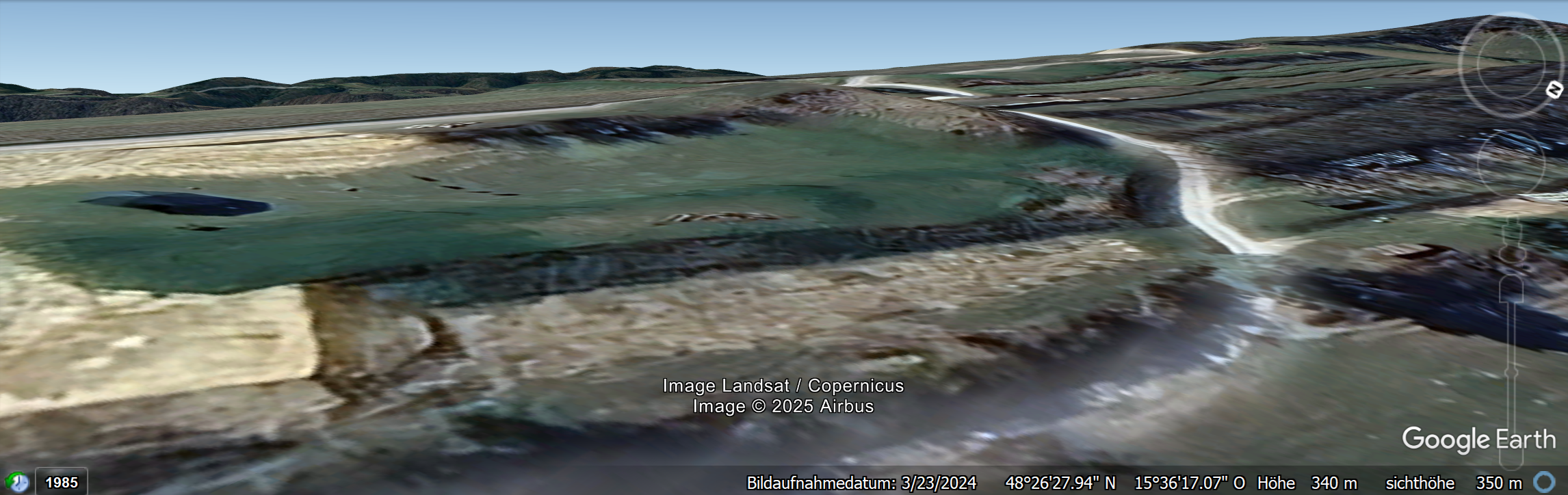
However, In many cases I could not find the exact location or the samples where from to many nearby locations to distinguish between them reasonably. Then, I used just rough coordinates and added an “~” character before them in the YAML file.

There are multiple map services that can be used for investigations. I prefer Google Earth Pro Desktop as it provides close 3D views of landscapes with a good resolution and you can get set pins and comment them what makes the detective work all the better.

How to create the interactive map

I split the processing of the YAML files and the creation of the interactive map into two R scripts:

1. Compile the data: Import all files using the package yaml, add additional data from the CrossRef database via the R package rcrossref, parse the GPS data into a uniform format, and save the resulting R object.

2. Create the interactive map: Build HTML pop-up windows for each pair of GPS coordinates, define the style of the corresponding point on the map and create the map as HTML widget using the package leaflet.

The reason for splitting the R scripting is simple: Compiling the database can take a while and may result in an error if I make changes to the YAML files. Therefore, I don’t want to compile it every time I experiment with the map style.

R Script 1: Compile the database

The full R script is available at github.com/DirkMittelstrass/QuaMap/R code/01_read_YAML_and_CrossRef.R

Handle GPS coordinates

One tricky part is importing the GPS coordinates. The package leaflet that I will use to create the map later does not accept the usual arc coordinate style, such as 51°11’10.73”N, but requires a numeric position, such as 51.18631. I could not find a package that would perform this conversion, so I asked ChatGPT to write a function for me, which it did:

library(stringr) # for manipulating strings

# Function for parsing GPS coordinates into leaflet-readable numeric format
convert_coordinate <- function(coordinate) {
  
  # If the GPS position is already stored as decimal, no action is needed
  if(is.numeric(coordinate)) return(coordinate)
  
  # The imprecision-marker is handled elsewhere
  if (str_starts(coordinate, "~") == TRUE)
    coordinate <- str_remove(coordinate, "~")
  
  # Now we split the string to a vector.
  # For example: 27°42'29"N  becomes c(27, 42, 29, "N")
  coord_vector <- str_split_1(coordinate, "°|’|'|\"")
  
  # Cycle through the vector and transform arc values into decimals
  decimal <- 0
  for (i in 1:length(coord_vector)) {
    
    # Stop cycle if geographic direction is reached ...
    if (str_detect(coord_vector[i], "N|S|E|W")) {
      
      # ... but flip sign if necessary
      if (coord_vector[i] == "S" | coord_vector[i] == "W")
        decimal <- -decimal
      
      break
    }
    decimal <- decimal + as.numeric(coord_vector[i]) / (60^(i-1))
  }
  return(decimal)
} 

Import YAML data

Reading all YAML files is quite easy if you use the yaml package. However, in case their is a formatting error breaking the YAML import, the package throws an exception. Thus, I put a tryCatch() block around the import of each file to not break the whole script.

Important information like the title of the publication, the list of authors and the name of the journal are not saved in the YAML. That is because I fetch them directly from the CrossRef server via the rcrossref package. The server is sometimes quite slow, don’t wonder if the fetching may take a while.

library(yaml) # for loading the database files
library(rcrossref) # for getting further information from the DOIs

# The path to the folder where your YAMLs are stored
database_directory <- "D:/00_Misc/QuaMap/publication library/"

# Get the paths of all YAML files
yaml_files <- list.files(database_directory, 
                         pattern = "\\.yaml$", 
                         full.names = TRUE)

# Remove elements containing the substring "_template"
yaml_files <- yaml_files[!grepl("_template", yaml_files)]

# Define empty list to fill in database entries
publications <- list()

# Cycle through all YAML files
for (yaml_file in yaml_files) {
  
  # Load YAML file in try block
  tryCatch(
    {
      # This might take a while and errors may be throw. 
      # Thus, print the current YAML file in the console
      current_file <- tools::file_path_sans_ext(basename(yaml_file))
      cat(current_file, "\n")
      
      # Attempt to load the YAML file
      paper <- yaml.load_file(yaml_file)
      
      # Use the file name also to extract the citation and the publishing year
      paper$FileName  <- current_file
      paper$Citation <- sub(".*-\\s(.*?)\\s-.*", "\\1", current_file)
      
      # Extract middle part of file name,
      # for example "rsos - Key et al. (2022) - Fordwich, UK"
      paper$Citation <- str_split_1(current_file, " - ")[2] 
      
      # Now get the "2022" from "Key et al. (2022)"
      paper$Year <- str_split_1(paper$Citation , "\\(|\\)")[2]
      
      # Fetch metadata from CrossRef
      metadata <- cr_works(paper$DOI)$data
      
      # Save the most important metadata in the publication list
      paper$Authors <- metadata$author[[1]]
      paper$Journal <- metadata$short.container.title
      paper$Title <- metadata$title
      
      for (i in 1:length(paper$Positions)) {
        
        # Convert coordinates to a leaflet-readable format
        gps_point <- paper$Positions[[i]]
        paper$Positions[[i]]$Latitude <- convert_coordinate(gps_point$Latitude)
        paper$Positions[[i]]$Longitude <- convert_coordinate(gps_point$Longitude)
        
        # Determine whether exact coordinates are given
        paper$Positions[[i]]$Precision <- "High"
        if (str_starts(gps_point$Latitude, "~") || 
            str_starts(gps_point$Longitude, "~"))
          paper$Positions[[i]]$Precision <- "Low"
      }
      
      # Add the files content to the publication list
      publications[[current_file]] <- paper
      
    }, # If something went wrong, ignore this YAML file
    error = function(e) {
      
      # Print the error message including the file name
      message(sprintf("Error: Failed to load the YAML file '%s'.", yaml_file))
      message("Error details: ", e$message)
    }
  )
}
cat("\n", length(publications), "YAML files loaded successfully.\n")

Save data as R object

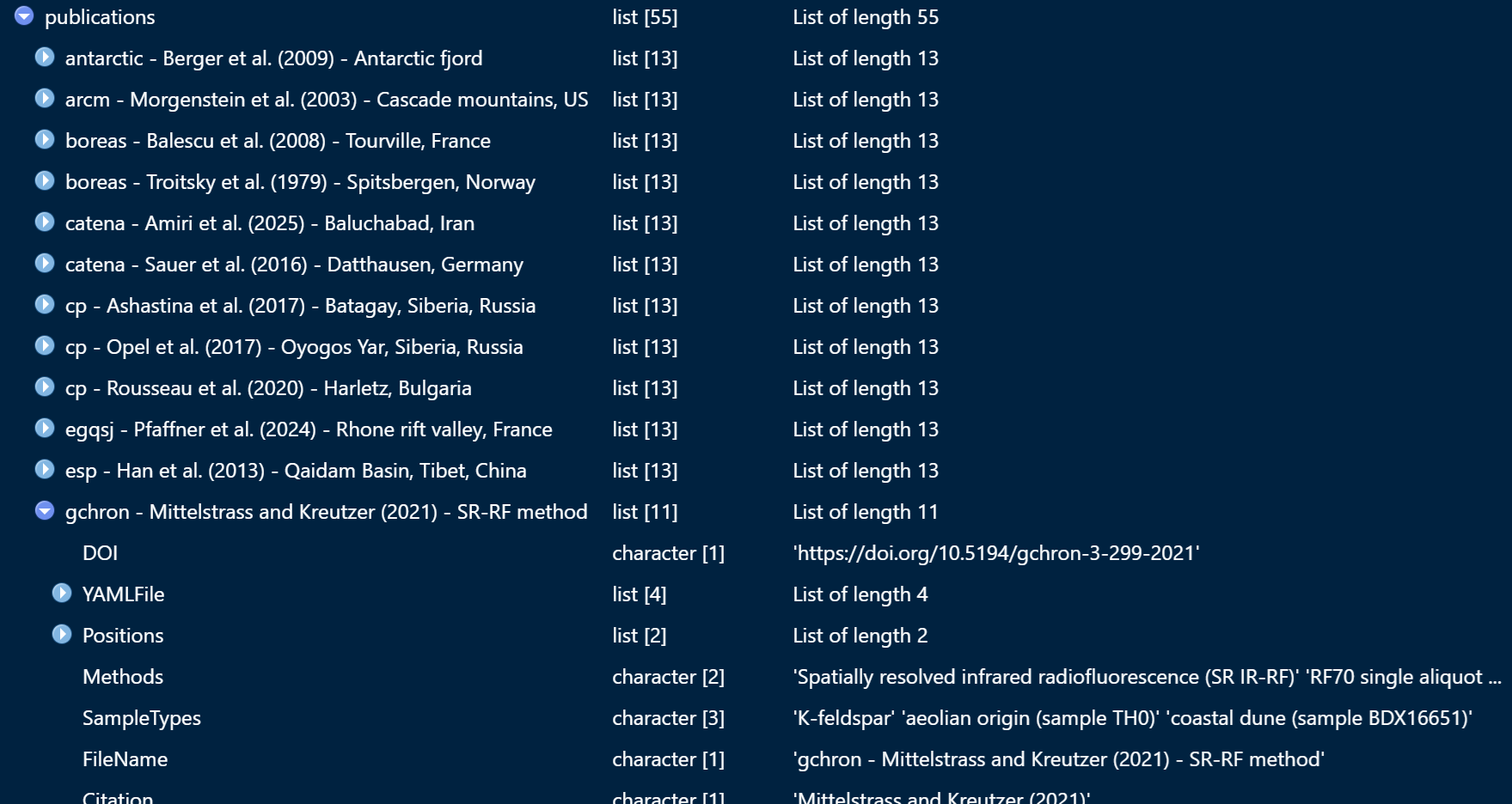
The script returns one big list object which looks like this:

Let us save the object .Robj file so we don’t have to re-run the script if parameters are changed when building the interactive map.

# Save the publication list as an R object
data_filepath <- paste0(database_directory, format(Sys.time(), "%Y-%m-%d"),"_quamap_database.robj")
saveRDS(publications, data_filepath)

R Script 2: Create the map

The second script performs three functions: Firstly, it creates informative mini-HTML pages for all GPS coordinates the database. Secondly it sets point styles and puts all GPS points into one data.frame. Thirdly, it creates the map by loading the chosen OpenStreetMap map and defining the data.frame of points as an overlay.

The full R script is available at: github.com/DirkMittelstrass/QuaMap/R code/02_build_map.R

Define HTML pop-ups

We will display the title and a link to the publication alongside the AI-extracted information in small pop-up windows, which will appear when a user clicks on them:

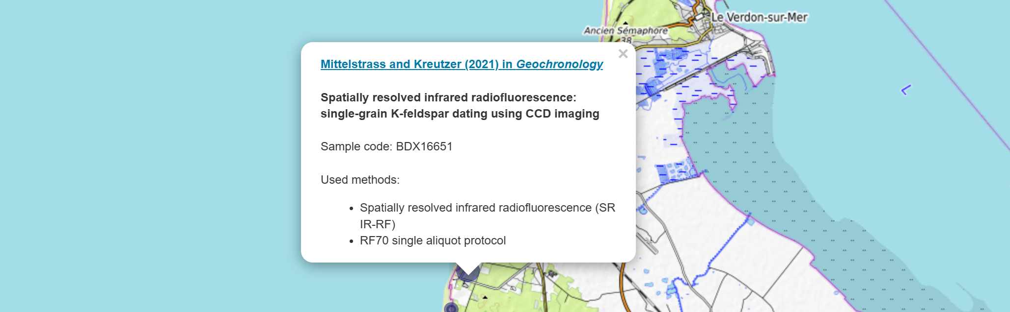
The pop-up shown is actually an HTML page that was dynamically created based on the database content. Therefore, we need to write some HTML code in our R script. This is made easier if we create a design template outside of R first:

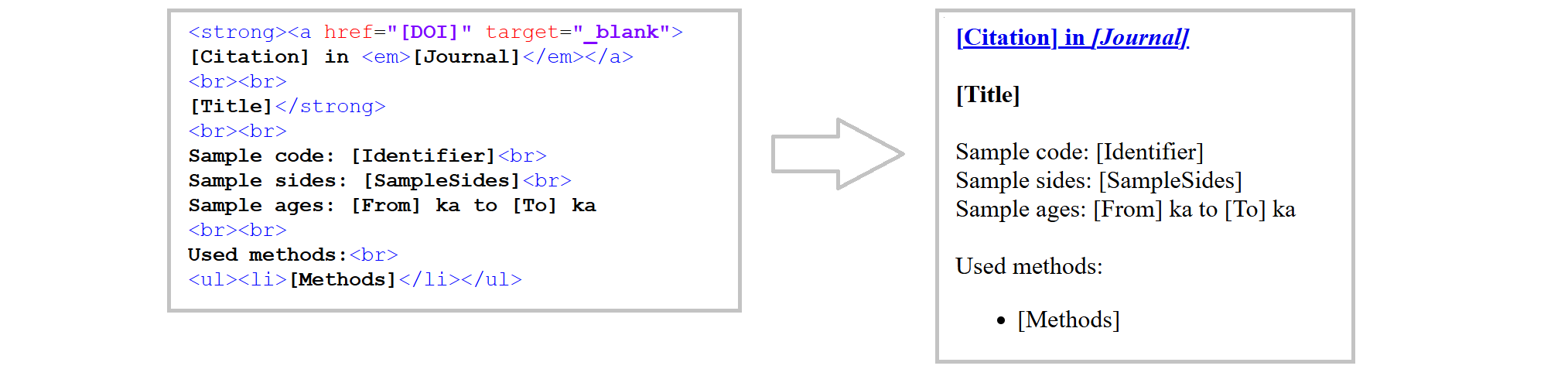
I recommend using an online editor for writing the HTML code. I used Code Pen, but there are plenty of other options out there. Alternatively, you can use a text editor and save the document as an HTML file.

The HTML template is available at: github.com/DirkMittelstrass/QuaMap/R code/pop_up_template.html

Next, we need to parse the HTML code as a text string in our R script and insert the database information dynamically. I suppose ChatGPT could write a complex function to do this automatically, but I decided to write one myself.

# Function for creating and formatting the HTML pop-up window
get_popup <- function(citation, 
                      journal, 
                      DOI, 
                      title, 
                      sample_code, 
                      sample_sides,
                      age, 
                      methods) {

  # Header
  popup <- paste0('<strong><a href="', DOI, '" target="_blank">', citation, 
                  ' in <em>', journal, '</em></a><br><br>', title, '</strong><br><br>')

  # Sample code
  if(!is.null(sample_code)) 
    popup <- paste0(popup, 'Sample code: ', sample_code, '<br>')
  
  # Sample sides
  if(!is.null(sample_sides)) 
    popup <- paste0(popup, 'Sample sides: ', sample_sides, '<br>')
  
  # Age range
  if(!is.null(age) && is.numeric(age$From) && is.numeric(age$To))
    popup <- paste0(popup, 'Sample ages: ', age$From, ' ka to ',age$To, ' ka<br>')
  
  # List of methods
  if(!is.null(methods) && length(methods) > 0) 
    popup <- paste0(popup, '<br>Used methods:<br><ul>',
                    paste0('<li>', methods, '</li>', collapse = ""), '</ul>')
  
  return(popup)
}

Set map points

First, we define a function that sets the colour of the points depending on the publication year. We could also change other point attributes, such as size or opacity. Alternatively, we could use different parameters, such as sample age or the methods used, to define the point parameters:

# Function for defining the point color
year_to_color <- function(year) {
  
  color_old <- "grey20"
  color_young <- "darkblue"
  start_year <- 2000
  current_year <- as.numeric(format(Sys.Date(), "%Y"))  # Get the current year
  
  if (year < start_year) return(color_old)
  if (year > current_year) return(color_young)
  
  # Create a gradient
  num_years <- current_year - start_year + 1
  colors <- colorRampPalette(c(color_old, color_young))(num_years)

  return(colors[year - start_year + 1])
}

We now load the database created in Script 1 and build a table of map points. Each point has its own pop-up window and is based on the GPS coordinates stored in the database:

# The path where your .Robj file is stored
database_directory <- "D:/00_Misc/QuaMap/publication library/"
database_name <- "2026-01-06_quamap_database.robj"

# Load the output from script 1
puplications <- readRDS(paste0(database_directory, database_name))

# Cycle through all available GPS coordinates
points <- review_table <- data.frame(NULL)
for (paper in puplications) {
  for (point in paper$Position) {
    
    # Get the popup
    popup <- get_popup(paper$Citation, 
                       paper$Journal, 
                       paper$DOI,
                       paper$Title, 
                       point$Identifier, 
                       point$SampleSides,
                       paper$AgeRange, 
                       paper$Methods)
    
    # Define the point color
    point_color <- year_to_color(as.numeric(paper$Year))
    
    # Define the point style
    if (point$Precision ==  "High") {
      point_size <- 5
      point_stroke <- TRUE
    } else {
      point_size <- 12
      point_stroke <- FALSE
    }
    
    # Add this point to the point table
    points <- rbind(points, data.frame(Latitude = point$Latitude, 
                                       Longitude = point$Longitude, 
                                       Popup = popup,
                                       Color = point_color,
                                       Size = point_size,
                                       Stroke = point_stroke))
  }
}

Initialize map

The map is created using the excellent leafmap package which uses map tiles from an user-defined OpenStreetMap server. If no server is defined, the default OpenStreetMap map tiles are used instead. A list of available other tile sets is provided at OpenStreetMap wiki. Please note that some servers are commercial and registration is required, while others are free but can be slow, such as OpenTopoMap which we will use in this example.

library(leaflet) # for creating the map

# Define the map object
map <- leaflet(points) %>%
  
  # Set the tile set server here or use addTiles() without
  # arguments to use the standard OpenStreetMap map
  addTiles(urlTemplate = "https://{s}.tile.opentopomap.org/{z}/{x}/{y}.png") %>%
  
  # Location and zoom at start
  setView(0, 50, zoom = 3) %>%
  
  # Overlay definition
  addCircleMarkers(
    ~Longitude, ~Latitude,  
    popup = ~Popup,
    radius = ~Size,  
    color = ~Color,
    fillOpacity = 0.5,
    stroke = ~Stroke
  )

Display or save the map

The map is provided as a JavaScript widget that can be embedded in an RMarkdown or Quarto HTML document, or on a webpage like this one. It can also be displayed directly in the RStudio output window.

# Display the map
map

We can also save the map as an HTML file using the htmlwidgets package. However, a connection to the internet is needed for this to work, as the OpenStreetMap tiles are loaded dynamically.

library(htmlwidgets) # for saving the map as HTML file 

# Define path of the HTML file ...
map_filepath <- paste0(database_directory, "qua_map.html")

# ... and save it there
saveWidget(map, file = map_filepath, selfcontained = TRUE)

The map we just created is available HERE.

Copyright and Fair Use

All data taken from scientific journal publications is subject to copyright law. Therefore, if the publications do not belong to you, there is always a risk of committing copyright infringement. The same applies if you use AIs to extract information, particularly given that these AI capabilities affect the business model of scientific publishers. An earlier version of the Quaternary map contained neat 50-word AI-generated summaries of the paper’s findings in the YAML files and pop-ups. However, I removed these short abstracts before publishing my work online to avoid receiving any letters from lawyers.

However, if you use data extracted from published work in a new context or for educational purposes, as I have done here, your work should be protected by Fair Use regulations.

To qualify as fair use, two main factors must be met:

• The use must be ‘transformative’, meaning it must be used for a purpose other than the original, or in a new context; it cannot simply be a ‘substitute’ for the original.

• The kind and amount of the use must be appropriate, i.e. it must be short.

However, I’m not a lawyer, and there is a lot of ambiguity about what is and isn’t allowed. Therefore, please don’t take what I have written as gospel. If you would like to find out more, I recommend the Fair Use portal of the American Library Association.

© Dirk Mittelstraß, 2020 - 2026 | This website was created with Rmarkdown