OSLdecomposition tutorial
1 Introduction
OSLdecompostion is a function library for the
statistical open-source programming language R. It is designed
to separate the signal components in continuous-wave optically
stimulated luminescence (CW-OSL) of quartz minerals, a standard method
for dating samples with an age between a few thousand and about 200.000
years. However, resulting ages might be biased by unstable signal
components as described by Bailey et al. (1997) and others. For readers
unfamiliar with this issue, chapter 5 and 6 in Preusser et al. (2009)
might be a good starting point. This software package shall give
scientific users the tools at hand to identify the the signal components
in their samples and to separate the long-term stable signals from the
unstable signals, thus to improve the reliability and accuracy of their
dating results. For a quick sum-up of what the package does, scroll
through my talk
I gave at the DLED 2019.
While this package was programmed for CW-OSL measurements of quartz in mind, it might also prove itself useful for other types of measurements. For example, some preliminary tests for multiple dating methods of feldspar samples showed interesting first result (I would love to see a publication investigating signal components in feldspar IRSL using my package). Another application might be for OSL dosimetry with artificial samples like Al2O3 or BeO.
2 Software environment
2.1 Installation
If you use RStudio,
you can install OSLdecomposition with the package manager
directly from the CRAN server. If you use R directly
via console or via another environment, simply execute the following
line of R code:
2.2 Dependencies
One main purpose of the package is to work as an extension of the extensive and excellent R package Luminescence, which is the de-facto standard for data analysis in the field of luminescence dating. You can learn more about the world of R packages for luminescence dating on Sebastian’s webpage r-luminescence.org. Other important packages deployed by OSLdecomposition are for example RMarkdown for automatically creating reports of the automatized analysis of SAR-protocol compatible data sets and DEoptim for to perform the genetic evolution of parameters during optimization tasks.
However, the necessary packages are installed automatically when
installing OSLdecomposition. An exception is
kableExtra which is used to create nicer tables in the
automatically created reports. However, kableExtra had its
issues with Linux, so its optional and not automatically installed.
2.3 Running at Linux
Regarding Linux, OSLdecomposition and its dependencies
run quite well on Linux but you might need to install some not-standard
system libraries. For Ubunutu 20.04 (and distributions based on it) you
can find here
a guide for getting OSLdecomposition and
Luminescence running on it. For other distributions, this
more
general guide might help you.
3 SAR data analysis tutorial
The single aliquot regenerative dose (SAR) protocol by Murray and
Wintle (2000) is the default measurement and analysis protocol of CW-OSL
measurement of quartz. The OSLdecomposition package
contains functions to make analysis of SAR data sets especially easy.
Those function have the prefix RLum.OSL_. The following
script examples describe how to perform a signal component-wise data
analysis for such a data set.
We recommend to copy & paste the code examples into a R script and run it once to see what happen. Then customize the script the way we describe it in the following sections.
3.1 Script example
# Load R packages
library(OSLdecomposition)
library(Luminescence)

# Load example data from the Luminescence package
data(ExampleData.BINfileData, envir = environment())
data_set <- Risoe.BINfileData2RLum.Analysis(CWOSL.SAR.Data)

# Check the data for consistency and shorten the measurement duration
data_set <- RLum.OSL_correction(data_set)

# Identify the OSL components globally (Step 1)
data_set <- RLum.OSL_global_fitting(data_set)

# Separate OSL components in each record
data_set <- RLum.OSL_decomposition(data_set)

# Calculate the equivalent doses for the fast component
De_fast <- analyse_SAR.CWOSL(data_set, OSL.component = 1)

# ... and also for the medium component
De_medium <- analyse_SAR.CWOSL(data_set, OSL.component = 2)

# Compare both in a kernel density plot
plot_KDE(list(De_fast, De_medium))
The output will look like this:
> # Load example data from the Luminescence package
> data(ExampleData.BINfileData, envir = environment())
> data_set <- Risoe.BINfileData2RLum.Analysis(CWOSL.SAR.Data)
> # Check the data for consistency and shorten the measurement duration
> data_set <- RLum.OSL_correction(data_set)
CORRECTION STEP 1 ----- Check records for consistency in the detection settings -----
All OSL records have the same detection settings
(time needed: 1.28 s)
CORRECTION STEP 2 ----- Cut records at specific time -----
Measurement duration of 336 records reduced to 20 s
(time needed: 0.1 s)
> # Identify the OSL components globally (Step 1)
> data_set <- RLum.OSL_global_fitting(data_set)
STEP 1.1 ----- Build global average curve from all CW-OSL curves -----
Built global average curve from arithmetic means from first 500 data points of all 336 OSL records
(time needed: 10.59 s)
STEP 1.2 ----- Perform multi-exponential curve fitting -----
Decay rates (s^-1):
Cycle Comp. 1 Comp. 2 Comp. 3 Comp. 4 Comp. 5 RSS F-value
K = 1 3.115 1.356e+06 Inf
K = 2 3.456 0.05745 5.802e+04 5551
K = 3 4.006 1.25 0.02935 2966 4585
K = 4 4.908 2.664 0.4329 0.01578 327.3 1983
K = 5 5.342 3.024 0.9848 0.2568 0.009924 292.8 28.83
Left loop because F-test value (F = 28.83) fell below threshold value (F = 150)
-> The F-test suggests the K = 4 model
Photoionisation cross sections (cm^2):
Cycle Comp. 1 Comp. 2 Comp. 3 Comp. 4 Comp. 5
K = 1 3.76e-17
K = 2 4.17e-17 6.94e-19
K = 3 4.84e-17 1.51e-17 3.54e-19 (Slow2)
K = 4 5.93e-17 3.22e-17 5.23e-18 (Medium) 1.91e-19 (Slow2)
K = 5 6.45e-17 3.65e-17 1.19e-17 3.1e-18 (Medium) 1.2e-19 (Slow2)
-> Most known quartz OSL components found in the K = 4 model
(time needed: 108.59 s)
> # Separate OSL components in each record
> data_set <- RLum.OSL_decomposition(data_set)
STEP 2.1 ----- Define signal bin intervals -----
Find intervals with lowest component cross correlation by maximising the denominator determinant in Cramers rule:
Maximum determinant = 0.1377 with interval dividing channels at i = 10, 73
(time needed: 1.13 s)
STEP 2.2 ----- Decompose each OSL curve -----
Calculate signal intensity n in each OSL by ' det+nls ' algorithm with empiric error estimation
Table of input decay constants and signal bin intervals for [decompose_OSLcurve()]:
name lambda t.start t.end ch.start ch.end
1 Component 1 4.00622665 0.00 0.40 1 10
2 Component 2 1.25030289 0.40 2.92 11 73
3 Slow2 0.02934643 2.92 20.00 74 500
........................
Successfully decomposed 336 records
(time needed: 11.19 s)
> # Calculate the equivalent doses for the fast component
> De_fast <- analyse_SAR.CWOSL(data_set, OSL.component = 1)
[plot_GrowthCurve()] Fit: EXP (interpolation) | De = 1875.01 | D01 = 1989.56
[plot_GrowthCurve()] Fit: EXP (interpolation) | De = 1532.6 | D01 = 2177.44
[plot_GrowthCurve()] Fit: EXP (interpolation) | De = 1386.16 | D01 = 2076.68
... (output shortened)
> # ... and also for the medium component
> De_medium <- analyse_SAR.CWOSL(data_set, OSL.component = 2)
[plot_GrowthCurve()] Fit: EXP (interpolation) | De = 539.85 | D01 = 913.61
[plot_GrowthCurve()] Fit: EXP (interpolation) | De = 911.61 | D01 = 1078.48
[plot_GrowthCurve()] Fit: EXP (interpolation) | De = 2046.94 | D01 = 1062.6
... (output shortened)
> # Compare both in a kernel density plot
> plot_KDE(list(De_fast, De_medium)) 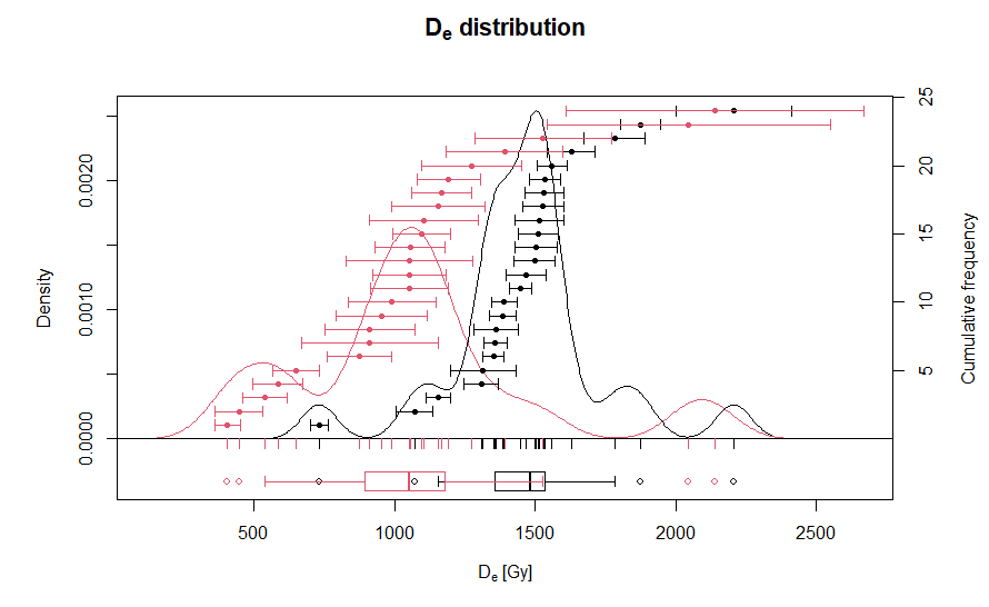 In the output diagram, black data
points are Fast component equivalent dose values and red data points are
Medium component equivalent dose values.
In the output diagram, black data
points are Fast component equivalent dose values and red data points are
Medium component equivalent dose values.
3.2 Analyse your own data set
To read a BIN or BINX data file, replace
code lines 5 to 7 of the script above with:
# Chose input file and convert it into a RLum.data object
file_path <- file.choose()
data_set <- read_BIN2R(data_set, fastForward = TRUE)
You can also read XSYG files by using
read_XSYG2R().
3.3 Automatically created reports
You can activate the output of detailed reports for the component
identification and separation steps with the parameter
report. Replace code line 12 to 16 with the following code
snippet:
# Identify the OSL components globally (Step 1)
data_set <- RLum.OSL_global_fitting(data_set, report = TRUE)

# Separate OSL components in each record
data_set <- RLum.OSL_decomposition(data_set, report = TRUE)
For each step, a new tab with the analysis report will automatically open in your browser. Examples for another data set can be found can be found here and here.
As default, these reports are not saved and will be deleted the
moment you end your R session. To save them as HTML file,
define the parameter report_dir with an directory path of
your choice. Be aware, that R does not accept “\” as folder separator.
You have to use either “/” or “\\”. The following code will save the
reports into your input file directory (see section 1.2):
# Identify the OSL components globally (Step 1)
data_set <- RLum.OSL_global_fitting(data_set, report = TRUE, report_dir = file_path)

# Separate OSL components in each record
data_set <- RLum.OSL_decomposition(data_set, report = TRUE, report_dir = file_path)
If you want to save the reports to your desktop, add this code line (might not work on all systems):
Per default, the report diagrams are saved as PDF vector graphics
into the subfolder /report_figures. You can change the
image output format by setting the parameter
image_format:
# Separate OSL components in each record
data_set <- RLum.OSL_decomposition(data_set, report = TRUE, report_dir = file_path, image_format = "jpg")
3.4 Photo-ionisation cross sections
The function RLum.OSL_global_fitting() estimates the
photo-ionisation cross section values of the signal components and
compares it with literature values for quartz. The requirement for
correct cross section values is, that the stimulation wavelength and the
stimulation stimulation intensity are specified correctly. Default
values are stimulation.wavelength = 470 (nm) and
stimulation.intensity = 35 (mW/cm²). In the example script,
the default stimulation intensity is too low. We estimate from figure 2
in the auto-report that 75 mW/cm² should be about right:
We obtain better suiting photoionisation cross section values:
Photoionisation cross sections (cm^2):
Cycle     Comp. 1              Comp. 2              Comp. 3              Comp. 4              Comp. 5
K = 1    1.76e-17
K = 2    1.95e-17 (Fast)      3.24e-19 (Slow2)
K = 3    2.26e-17 (Fast)      7.05e-18 (Medium)    1.65e-19 (Slow2)
K = 4    2.77e-17 (Fast)      1.5e-17              2.44e-18             8.89e-20
K = 5    3.01e-17 (Fast)      1.7e-17              5.55e-18 (Medium)    1.45e-18 (Slow1)     5.59e-20
-> Most known quartz OSL components found in the K = 3 model
3.5 CW-OSL model selection
The single curve component separation function
RLum.OSL_decomposition() uses the 3-component-model (K
= 3) as default. You can change the used model manually with the
parameter K. In the above example, the K = 2 might
also lead to sufficient results. We can test this by setting:
For other data sets, the K = 3 model might not sufficiently describe the complexity of the CW-OSL decays and the K = 4 is a better choice. But be aware that precision and robustness against systematic errors of the decomposition process declines with an increasing number of components. The approach should be: As much as necessary, as little as possible
4 References
Bailey, R. M., Smith, B. W. and Rhodes, E. J., 1997. Partial bleaching and the decay form characteristics of quartz OSL, Radiation Measurements, 27(2), 123–136.
Kreutzer S, Burow C, Dietze M, Fuchs M, Schmidt C, Fischer M, Friedrich J, Mercier N, Philippe A, Riedesel S, Autzen M, Mittelstrass D, Gray H, Galharret J (2022). Luminescence: Comprehensive Luminescence Dating Data Analysis_ R package version 0.9.19, https://CRAN.R-project.org/package=Luminescence.
Murray, A.S., Wintle, A.G., 2000. Luminescence dating of quartz using an improved single-aliquot regenerative-dose protocol. Radiation Measurements 32, 57–73. https://doi.org/10.1016/S1350-4487(99)00253-X
Preusser, F., Chithambo, M.L., Götte, T., Martini, M., Ramseyer, K., Sendezera, E.J., Susino, G.J., Wintle, A.G., 2009. Quartz as a natural luminescence dosimeter. Earth-Science Reviews 97, 184–214. https://doi.org/10.1016/j.earscirev.2009.09.006
© Dirk Mittelstraß, 2020 - 2026 | This website was created with Rmarkdown